Thomas-Fermi Theory

Accordingly, the slow spatial variations require the substitution $%% k_{F}^{2}\rightarrow \overline{k}_{F}k_{F}$ in (15), where $\overline{k}_{F}$ may be viewed as a variational parameter, the whole spatial variation being transferred upon the new Fermi wavevector $k_{F}$; a similar substitution $k_{F}^{3}\rightarrow \overline{k}_{F}^{2}k_{F}$ holds for the electron density (14), and it is worth noting that such substitutions are valid over those space regions where $\overline{k}_{F}$ and $k_{F}$ are comparable in magnitude; such substitutions are corrected by the quantal effects of the Hartree equations, as discussed above, as due to the abrupt spatial variations of the self-consistent potential and the electron density in the neighbourhood of the ionic cores. A linearized version[1] is thereby obtained for the Thomas-Fermi scheme, which consists in

$$\overline{k}_{F}k_{F}/2-\varphi =0\;\;,\;\;n=\overline{k}_{F}^{2}k_{F}/3\pi ^{2}=(q^{2}/4\pi )\varphi \;\;\;,$$ (17)

according to (14) and (15), where the Thomas-Fermi screening wavevector $q$ has been introduced through

$$q^{2}=\frac{8}{3\pi }\overline{k}_{F}\;\;;$$ (18)

it will be taken as the variational parameter; the Bohr radius $a_{H}=\hbar ^{2}/me^{e}=0.53$Å is used as length unit and the atomic unit $%% e^{2}/a_{H}=27.2$eV is also used for energy. Poisson's equation (7) reads now

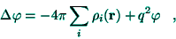$$\Delta \varphi =-4\pi \sum_{i}\rho _{i}({\bf r})+q^{2}\varphi \;\;\;,$$ (19)

and its solution provides the self-consistent field $\varphi$. It is worth noting that the quasi-classical description and the quasi-classical equilibrium equation (15) are valid for slow spatial variations, requiring thus the linearized Thomas-Fermi scheme; the usual ''$3/2$''-Thomas-Fermi model, where $n\sim \varphi ^{3/2}$, would be inappropriate for the slightly inhomogeneous electron liquid; the ''$3/2$''-Thomas-Fermi model holds in the classical limit of the quantal mechanics, which is often called the ''quasi-classical approximation''.[2]$^{,}$[4]

Two-cluster aggregation

In order to estimate the effect of the quantal corrections, as arising from those spatial regions of abrupt variations, the variational parameter $\overline{k}_{F}$ given by (18) (associated with the electron density) may be compared with the average Fermi wavevector

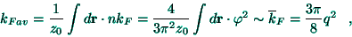$$k_{Fav}=\frac{1}{z_{0}}\int d{\bf r}\cdot nk_{F}=\frac{4}{3... ...hi ^{2}\sim \overline{k}_{F}=\frac{3\pi }{8}%% q^{2}\;\;\;,$$ (20)

where

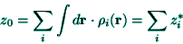$$z_{0}=\sum_{i}\int d{\bf r}\cdot \rho _{i}({\bf r})=\sum_{i}z_{i}^{*}$$ (21)

is the total charge; it is worth noting here the electric neutrality of the aggregate, as obtained from Poisson's equation (7), for instance; such a comparison can also be made between the variational parameter $q$ and the average parameter $q_{av}$, obtained through (18) with $\overline{k}%% _{F}$ replaced by $k_{Fav}$.